A20 - Neural Networks

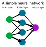
Neural network is a mathematical model that mimics brain function. It is made up of interconnecting artificial neurons (programming constructs that mimic the properties of biological neurons) in a similar manner shown below.

http://upload.wikimedia.org/wikipedia/en/thumb/1/1d/Neural_network_example.png/180px-Neural_network_example.png

In this activity, we use neural networks as a method to classify objects into classes depending on the extracted features. We again use pillows and kwek-kwet data set from activity19. The features used are ROI pixel area, length-to-width ratio, average red component (NCC) and average green component (NCC).

A code was already prepared by Jeric Tugaff and was only modified for this activity's purpose. The values used are as 4 input feature vectors (normalized between 0-1) both from 4 training objects for each class and 4 test objects for each class.

The neural network is trained using the training set. The code is expected to output values close to

[0 0 0 0 1 1 1 1]

meaning the first four test object will be classified as belonging to the pillows class and the second set of test objects will be classified under the kwek-kwek class. The output is as follows. From this table, 100% classification of the test objects is obviously obtained.

//code
chdir('C:\Documents and Settings\VIP\Desktop\ap186\A20');

training = fscanfMat('training.txt');
test = fscanfMat('test.txt');

//training
mntr = min(training, 'c');
tr2 = training - mtlb_repmat(mntr, 1, 8);
mxtr = max(tr2, 'c');
tr2 = tr2./mtlb_repmat(mxtr, 1, 8);

//test
mnts = min(test, 'c');
ts2 = test - mtlb_repmat(mnts, 1, 8);
mxts = max(ts2, 'c');
ts2 = ts2./mtlb_repmat(mxts, 1, 8);

tr_out = [0 0 0 0 1 1 1 1];
N = [4, 10, 1];
lp = [0.1, 0];
W = ann_FF_init(N);

T = 400;
W = ann_FF_Std_online(tr2,tr_out,N,W,lp,T);
//x is the training t is the output W is the initialized weights,
//N is the NN architecture, lp is the learning rate and T is the number of iterations

// full run
ann_FF_run(ts2,N,W) // classification output

//end code

---
Thanks Jeric Tugaff for helping me understand how neural network works and for helping me with the program.

---
Rating 7/10 since I implemented the program correctly but was very dependent on Jeric's tutorial and discussion. :)

A19 - Probabilistic Classification

Linear discriminant analysis is a classification technique by which one creates a discriminant function from predictor variables.

In discriminant analysis, there is a dependent variable (Y) which is the group and the independent variables (X) which are the object features that might describe the group. If the groups are linearly separable, then we can use linear discriminant analysis. This method suggests that the groups can be separated by a linear combination of features that describe the objects.

In this activity, i used LDA to classify pillows (chocolate-coated snack) and kwek-kwek (orange, flour-coated quail egg) based on the features such as pixel area, length-to-width ratio, average red component (NCC), and average green component (NCC).

Images of the two samples were taken using Olympus Stylus 770SW. The images are then white balanced using reference white algorithm with the white tissue as the reference. This is to maintain uniform tissue color in each of the images. The images are then cut such that a single image contains a single sample. Features are then extracted from each of the cut images in the same manner as the previous activity.

The data set is again divided into training and test sets, with the first four images of each sample comprising the training set while the last four images for the test set.

Following the discussion and equations from Pattern_Recognition_2.pdf by Dr. S. Marcos, I computed the following values.

An object is assigned to a class with the highest f value. As can be seen from the table below, most of group 1 (pillows) have higher f1 values while those in group 2 (kwek-kwek) have higher f2 values. 100% classification is obtained.

---
//code

TRpillow=fscanfMat('TrainingSet-Pillows.txt');
TSpillow=fscanfMat('TestSet-Pillows.txt');

TRkwek=fscanfMat('TrainingSet-Kwekkwek.txt');
TSkwek=fscanfMat('TestSet-Kwekkwek.txt');

TRpillow=TRpillow';
TSpillow=TSpillow';
TRkwek=TRkwek';
TSkwek=TSkwek';

TRpilmean=mean(TRpillow,1);
TRkwekmean=mean(TRkwek,1);

globalmean=(TRpilmean+TRkwekmean)/2;
globalmean=mtlb_repmat(globalmean,4,1);

TRpillow=TRpillow-globalmean;
TRkwek=TRkwek-globalmean;

c_pil=((TRpillow')*TRpillow)/4;
c_kwek=((TRkwek')*TRkwek)/4;

C=((4*c_pil)+(4*c_kwek))/8;
P = [0.5;0.5];
for i=1:4
f1(i) = (TRpilmean*inv(C)*(TSkwek(i,:)'))-((0.5)*(TRpilmean)*inv(C)*(TRpilmean')+log(P(1)));
f2(i) = (TRkwekmean*inv(C)*(TSkwek(i,:)'))-((0.5)*(TRkwekmean)*inv(C)*(TRkwekmean')+log(P(2)));
end

//end code

---
Thanks Jeric Tugaff for the tips and discussions and Cole Fabros for the images of the sample.

---
Rating 8.5/10 since I implemented and understood the technique correctly but was late in posting this blog entry.

A18 - Pattern Recognition

Pattern recognition, as a subtopic of machine learning, aims to classify data according to a statistical information extracted from its patterns.

A pattern is usually a group of measurements or observations extracted from the data set. In essence, a pattern is a set of quantifiable features. These features are then arranged into an ordered set to define a feature vector. Feature vectors, then, define the grouping of the data into classes.

In pattern recognition, the specific goal is to decide if a given feature vector belongs to one of the several classes.

In this activity, we aim to classify a set of images into one of the four classes - kwek-kwek (orange, flour-coated quail egg), squid balls, piatos potato chips, pillows (chocolate coated snack).

Images of the four samples were taken using Olympus Stylus 770SW. The images are then white balanced using reference white algorithm with the white tissue as the reference. This is to maintain uniform tissue color in each of the images. The images are then cut such that a single image contains a single sample.

FEATURE VECTOR
For each of the individual sample, the features extracted are as follows:
1. pixel area
2. length-to-width ratio
3. average red component (NCC)
4. average green component (NCC)

To get the pixel area, the sample images were first binarized to separate ROI from the background. Closing operation is then performed on the binarized images to reduce effect of poor thresholding. The pixel area is then equal to the sum of the (binarized then closed) image.

Length-to-width ratio is computed as the maximum filled pixel coordinate along the x-axis minus the minimum filled pixel coordinate along x-axis divided by its y-axis counterpart.

The average red component and green component is obtained from the ROI only using Normalized Chromaticity Coordinates.

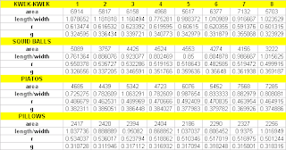
The following table summarizes the features extracted for all the sample images.

MINIMUM DISTANCE CLASSIFICATION
The data set is divided into two - training and test sets. The training set is composed of the first four images from each classes while the test set are the last four images for each sample.
(Note: Pixel Area was first normalized before subjecting to minimum distance classification.)

To facilitate classification of the test images into one of the four classes, we use minimum distance classification.

This is done by getting the mean feature vector from the training set for each class. Therefore, we get the mean of the training set by getting the mean pixel area, mean L/W, mean r, mean g for each of the four classes.

Classification is done by getting the Euclidean distance of an unknown feature vector from the mean feature vector of each class. The unknown feature vector then belongs to the class with which it has the smallest distance.

In this activity, we use the test set to check for the validity of minimum distance classification as a pattern recognition algorithm. The following results were obtained.

From the matrix above, it is shown that among the 16 samples of the test set, only 1 was misclassified as belonging to another class.

---
Thanks Benj for the discussions with regards to this activity and Cole for the sample images.

---
Rating: 8.5/10 since I implemented the task correctly but was late in posting this blog entry.

A16 - Color Image Segmentation

In image segmentation, a region of interest (ROI) is picked out from the rest of the image such that further processing can be done on it. Selection rules are based on features unique to the ROI.

In this activity, we use color as a feature for segmenting images. To do so, we first transform the color image's RGB into rgI. rgI is part of the normalized chromaticity coordinates or NCC color space. This color space separates chromaticity (r g) and brightness (I) information.

Per pixel, let I = R+G+B. Then the normalized chromaticity coordinates are

r = R/I
g = G/I
b = B/I

---



*http://images.replacements.com/images/images5/china/H/homer_laughlin_fiesta_shamrock_green_mug_P0000201549S0044T2.jpg

---
Parametric Probability Distribution

Segmentation based on color can be performed by determining the probability that a pixel belongs to a color distribution of interest. This implies that the color histogram of the region of interest must first be extracted. To do so, one crops a subregion of the ROI and compute the histogram from it. The histogram when normalized by the number of pixels is already the probability distribution function (PDF) of the color. To tag a pixel as belonging to a region of interest or not is to find its probability of belonging to the color of the ROI. Since our space is r and g we can have a joint probability p(r) p(g) function to test the likelihood of pixel membership to the ROI. We can assume a Gaussian distribution independently along r and g, that is, from the r-g values of the cropped pixel we compute the mean μr , μg and standard deviation σr , σg from the pixel samples. The probability that a pixel with chromaticity r or g belongs to the ROI is then

The joint probability is just the product of p(r) and p(g).

Shown below is the cropped region of the colored image, wherein we get the mean and standard deviation for both r and g so as to get the probability that a certain pixel belongs to the ROI.



We perform this over all pixels and plot the probability that a pixel belongs to our ROI.
Here's the distribution



And here's the segmented image, wherein the white parts corresponds to the pixels belonging to the ROI according to our Gaussian PDF.



---

Nonparametric Segmentation (Histogram Backprojection)

In non-parametric estimation, the histogram itself is used to tag the membership of pixels. Histogram backprojection is one such technique where based on the color histogram, a pixel location is given a value equal to its histogram value in chromaticity space.

Here's the histogram used

and the corresponding segmented image



Nonparametric image segmentation produced better results as compared to the parametric segmentation. Also, in nonparametric segmentation, we never assumed normality of distribution of the r and g, thus, this method is more accurate as compared to parametric segmentation.

---
Reference:
Activity 16 Lecture Handouts by Dr. Maricor Soriano.

---
Thanks to Ed for the valuable discussions and arguments with regards to the technique.

---
I give myself a 10 for I implemented image segmentation quite well. :)

A15 - Color Image Processing

A colored digital image is an array of pixels each having red, green and blue light overlaid in various proportions. Per pixel, the color captured by a digital color camera is an integral of the product of the spectral power distribution of the incident light source S(λ), the surface reflectance r(λ) and the spectral sensitivity of the camera η(λ).

Each pixel in a color image has R, G, B values, each of which has a balancing constant equal to the inverse of the camera output when the camera is shown a white object. This balancing constant is implemented through white balancing algorithm of a digital camera.
At its simplest - the reason we adjust white balance is to get the colors in your images as accurate as possible.*

More on white balancing at this link. *

---

The following images shows the effect of changing white balance on camera settings

WB: auto

sunny and cloudy settings

fluorescent and tungsten settings

From these images, we can obviously account that white doesn't appear white especially in tungsten settings. We therefore correct this image using the two algorithms we describe below.

---

AUTOMATIC WHITE BALANCING ALGORITHMS

There are two popular algorithms of achieving automatic white balance. The first is Reference White Algorithm and the second is the Gray World Algorithm.

In the Reference White Algorithm, you capture an image using an unbalanced camera and use the RGB values of a known white object as the divider.

In the Gray World Algorithm, it is assumed that the average color of the world is
gray. Gray is part of the family of white, as is black. Therefore, if you know the RGB of a gray object, it is essentially the RGB of white up to a constant factor. Thus, to get the balancing constants, you take the average red, green and blue value of the captured image and utilize them as the balancing constants.

original image (tungsten WB)


reference white algorithm

gray world algorithm

As can be seen from the images, the reference white is superior in terms of image quality. This is because in gray world algorithm, averaging channels puts bias to colors that are not abundant.
---

We also test this algorithm for an image with objects of the same hue.


original image (green objects under tungsten WB settings)

reference white algorithm

gray world algorithm

In these images, we see that the gray world algorithm is superior in terms of producing accurate colors. The green objects looks more green than in the reference algorithm.

---
Note: All images may look dark. This is because I used 0.7 exposure value to avoid saturation of images after processing them.

I give myself a 10 for I implemented the algorithms correctly. :)

---
Thanks to VIP's digital SLR camera. *nakisingit po ako sa experiment ni Ate Loren.*

A14 - Stereometry

Stereometry is another 3D reconstruction algorithm based on the human eye perception of depth. We perceive depth by viewing the same object at two different angles (two eyes separated by some distance).

In this activity, we explore how stereometry works. We try to reconstruct a 3D object using 2 images of taken by the same camera at the same distance z from the object but with a different x position (assuming x is the parallel axis between the camera and the object).

From this diagram, by simple ratio and proportion, depth z is perceived using the relation

(1)

If done on several points, we can reconstruct the 3D surface of the object.

The sample I used is a rubik's cube shown below with the tsai grid. (b=50mm, refer to diagram)

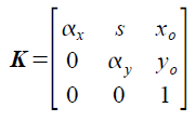
The camera used was first calibrated to get its internal parameter f (focal length). From the a's calculated using Activity 11 – Camera Calibration, matrix A is formed by recasting the a's. We then get the values of matrix A(1:3,1:3) and factorize this using RQ factorization, to get upper diagonal matrix K. (Note: Ensure that the factorized A(3,3) element is 1 by dividing the matrix by K(3,3)). The K-matrix obtained is shown below.

Knowing that K is just

and
we now have a value for focal length f (let kx=1);

We then get z values (using the equation 1) for different points on the object (purple dots).

Reconstruction was done using Matlab's griddata instead of SciLab's splin2d because of the latter's initial requirement of increasing values for both x and y image coordinates. Matlab's griddata function, however, works well for random values of x and y image coordinates.

Reconstruction of the rubik's cube is shown below.

It may not seem obvious but the reconstruction obtained the general height difference of the points selected. The edges are not defined but it somehow approximates the shape of the rubik's cube.

---
Thanks Cole for helping me with the images and JC for the discussions with regards to reconstruction.

---
Rating 6/10 since
1. reconstruction is not that good
2. I used Matlab in reconstruction rather than SciLab
3. I posted this blog very late.

A13 - Photometric Stereo

Photometric stereo is an algorithm for obtaining local surface orientation by using several images of a surface taken under different illumination conditions with the camera viewpoint held fixed.

The technique assumes that intensity I captured by camera at point (x,y) is directly proportional to brightness of surface at that point. This also assumes that light rays arriving on the surface are parallel. Shape of the surface is estimated from the multiple images and the information about the surface is coded in the shadings obtained from the images.

In this activity, we use Photometric Stereo technique to obtain a 3D reconstruction from 2D images. The input images are shown below.

The intensity at each point is denoted in matrix form as

Knowing the light source directions (V) for each of the input images (I), we use the equation below to solve for g.

From the computed values of g (a 3 row matrix corresponding to the xyz locations), we get a normal vector by dividing each element in a column with the magnitude of that column. After this, a linear integral was used to obtain the z values. Plotting z with a 128x128 plane yields the following 3D reconstruction.

---
Rating: 10/10 for the accurate reconstruction of the shape of the input images using the algorithm