A11 - Camera Calibration

In this activity we model the geometric aspects of image formation to recover information that was lost in the process of projecting brightness values from surfaces existing in 3D world space to 2D sensor space.

To do this, we first take a picture of a checkerboard pattern known as Tsai Grid.

Using SciLab's locate function, we selected 25 points on this image to get the pixel value of these points. We also take note of the real world coordinates of these points by letting the left side of the board to be the x-axis, the right side as the y-axis and the vertical as the z-axis. Each square has a side length of one inch. The origin is shown in pink below.

The green dots are the 25 points we've selected for our calibration. Next, we set up the matrix Q shown by equation below for values of i from 1 to 25. (i stands for image coordinate, o for real world object coordinate)

We then solve for a using equation below.




The resulting values of matrix a can then be used in the following equations to get the resulting 2D image coordinate by knowing the real world coordinates of the point. (a_34 is set to 1)

Implementing this method:

Real world coordinates of the green dots:
1. (8,0,12)
2. (6,0,10)
3. (2,0,10)
4. (4,0,9)
5. (6,0,8)
6. (6,0,3)
7. (4,0,2)
8. (2,0,3)
9. (6,0,5)
10. (4,0,3)
11. (0,8,12)
12. (0,5,10)
13. (0,2,10)
14. (0,5,8)
15. (0,3,7)
16. (0,5,4)
17. (0,7,2)
18. (0,2,1)
19. (0,3,3)
20. (0,5,1)
21. (0,0,1)
22. (0,0,3)
23. (0,0,5)
24. (0,0,6)
25. (0,0,11)

Corresponding Image Coordinates (Pixel Value)

point	y_image	z_image
1	23.214286	235.11905
2	53.571429	200
3	108.33333	205.35714
4	82.738095	185.11905
5	54.761905	163.09524
6	57.738095	73.214286
7	85.714286	63.095238
8	110.11905	86.904762
9	55.952381	108.92857
10	85.119048	80.357143
11	246.42857	236.90476
12	201.19048	202.38095
13	159.52381	205.95238
14	201.19048	166.66667
15	172.61905	152.97619
16	199.40476	80.357143
17	227.97619	55.952381
18	159.52381	55.357143
19	172.02381	85.119048
20	198.80952	45.238095
21	133.92857	60.714286
22	134.52381	92.261905
23	133.92857	125
24	133.33333	141.07143
25	132.7381	224.40476

Resulting matrix a

-13.2561
9.736856
-0.88994
134.7117
-4.07642
-4.2728
15.07773
45.71427
-0.01371
-0.01504
-0.00559

New image coordinates after using the matrix a

point	y_new	z_new
1	21.842763	235.67576
2	53.69017	199.59722
3	108.32033	205.44708
4	82.330771	184.49906
5	55.041758	162.50365
6	58.274085	73.794279
7	85.553674	63.772888
8	110.40641	86.620738
9	57.005504	108.60976
10	85.109881	80.396867
11	248.48566	236.84126
12	200.81792	201.5441
13	158.94669	205.61779
14	200.29104	164.72204
15	172.19655	151.17308
16	199.27642	93.813046
17	227.597	52.018523
18	158.96577	54.178965
19	171.88968	83.28296
20	198.54783	42.893636
21	134.57351	61.133497
22	134.29241	92.497568
23	134.00484	124.58259
24	133.85857	140.90327
25	133.10108	225.42079

Getting the difference between these computed values with the actual values gives the following mean values for each coordinate:
y: 0.474705
z: 1.365954

-o0o-
Collaborator: Cole Fabros

-o0o-
Grade: 10/10 since I implemented the camera calibration well, and that the mean difference for each axis is within one pixel. :)

A10 – Preprocessing Handwritten Text

In this activity we tried to extract handwritten text from an imaged document with lines. The image I used is shown below.

To remove the lines, I first obtained the FFT of this image.

The lines in the image are frequent, therefore, we can conclude that to remove the lines we need to suppress the frequencies that correspond to these lines.

The enhanced image after working on the Fourier space is shown below.

We then binarized this image for further cleaning process.

The image below is a result of performing opening operation on the binary image.

I repeated the same opening operation on the image, ad this results to the following image.

In both opening operations, the resulting image shows no success. The text are not readable. Part of the lines were even enhanced.

-o0o-
Thanks Ed for pointers and help in GIMP.

-o0o-
Rating: 5/10 since I was only able to remove the lines from the original image and that I wasn't successful in extracting the text from the image. The resulting image was also very dirty.

A9 - Binary Operations

The goal for this activity is to integrate everything we have learned so far to determine the best estimate of area (in pixel count) of simulated “cells”. We will also learn to use more morphological operators for enhancing and analyzing binarized images.

CLOSING and OPENING Morphological Operations
Opening is defined as an erosion followed by a dilation using the same structuring element for both operations. The basic effect of opening is somewhat like erosion in that it tends to remove some of the foreground (bright) pixels from the edges of regions of foreground pixels, but is less destructive. ***

Closing is defined as a dilation followed by an erosion using the same structuring element for both operations. Closing is similar in some ways to dilation in that it tends to enlarge the boundaries of foreground (bright) regions in an image (and shrink background color holes in such regions), but it is less destructive of the original boundary shape. ***

Getting Cell Area

The above image was first sampled by cropping 256x256 images. This was done because of two reasons. One is to save memory space since working with large images correspond to larger memory and two is to obtain an accurate value for the cell area by sampling on different regions of the image.

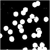
Below is a 256x256 cropped image. We first binarized this image to simplify the separation of background from region of interest (ROI). The optimum threshold can be found by examining the histogram of this image.

The binarized image is shown below.

Performing OPENING on the image results to the following image. The white pixels which are part of the background were removed.

Performing CLOSING operation results to the image below. Separation of touching blobs were observed.

We then use bwlabel function in SciLab to returns an image matrix which is of the same size as the original image but now containing labels for the connected objects in it. From this matrix, we can get the area of the cells since the each blob is a set of connected pixels.

We repeated the above procedures for different sample images and obtained a histogram of the cell area.

From this histogram, we can deduce that the pixel area of a cell in the image has a value between 500-550 pixels. Reducing the x-axis to 450-550 pixels shows the following histogram. This was done to limit the calculated area to those that best represents the cell area, since bins with smaller values can be accounted to small connected components, which is unlikely area of the cell.

We then get the mean and the standard deviation of the cell area obtained. The values were
area = 521.84444 pixels
std dev = 20.685915

We then checked if this values are correct. This was done by getting the cell area from an image with separated cells.

The values obtained are as follows
544.
527.
518.
535.
530.

Clearly, these values lie within the acceptable limit for the calculated area of the cell. The mean value obtained is thus correct. :)

-o0o-
Thanks Jeric for the tips on getting the histogram of the areas obtained.

-o0o-
I give myself a 10 for I implemented the necessary techniques well.

A8 - Morphological Operations

Morphology refers to shape or structure. In image processing, classical morphological operations are treatments done on binary images, particularly aggregates of 1's that form a particular shape, to improve the image for further processing or to extract information from it. All morphological operations affect the shape of the image in some way, for example, the shapes may be expanded, thinned, internal holes could be closed, disconnected blobs can be joined.

In this activity, we learned two basic morphological operations done on images --- DILATION and EROSION.

From Dr. Soriano's lecture notes, dilation is defined as follows.

On the other hand, erosion operator is defined as

From these definitions, we predicted the outcome of an image after dilating and eroding it with certain structuring elements.

We used the following binary images as test objects:

square (50×50)
triangle (base = 50 , height = 30)
hollow square (60×60, edges are 4 pixels thick)
plus sign (8 pixels thick and 50 pixels long for each line)
circle (radius 25)

The structuring elements used are shown below.
1. 4×4 ones
2. 4×2 ones
3. 2×4 ones
4. cross, 5 pixels long, one pixel thick.

We then check our predictions using SciLab's dilate and erode functions.

DILATION
The dilation results for each structuring element is shown below

EROSION
The erosion results for each structuring element is shown below

THIN
According to SciLab:
thin - thinning by border deletion
Function thin performs thinning of binary objects. It uses the Zhang-Suen, a de facto standard and simple technique. The resulting image, the skeleton, is not always connected and is very sensible to noise. For thin shapes, it should work faster and provide better quality. You will need some pruning criterium to eliminate spurs.

SKEL
According to SciLab:
skel - skeletonization, thinning, Medial Axis Transform
Function skel performs skeletonization (thinning) of a binary object. The resulting medial axis is multi-scale, meaning that it can be progressively pruned to eliminate detail. This pruning is done by thresholding the output skeleton image.
The algorithm computes skeletons that are guaranteed to be connected over all scales of simplification. The skeletons are computed using the euclidean metric. This has the advantage to produce high-quality, isotropic and well-centered skeletons in the shape. However the exact algorithm is computationally intensive.

-o0o-
Notes:
The predictions were visualized and written in a piece of paper. I'll try to scan them for posting and for comparison as well. For now, I could only say that some of my predictions, as to what the outcome of the image looked like after dilation and erosion using the given structuring elements, did not match the simulation done in SciLab. I would say 70% of my predictions were correct. I had difficulty especially with predicting images after erosion. Also, I wasn't so sure about my prediction in using the cross structuring element.
With all these reasons and knowing that I'd only predict roughly 70% of the outcome of the images, I give myself a 7/10 for this activity.

-o0o-
Collaborators:
Thank you JC Nadora, Jeric Tugaff, Toni Lei Uy, Benj Palmares, Cole Fabros, Ed David, Angel Lim, Mark Bejemino for the invaluable discussions regarding erosion and dilation, especially with prediction. More thanks to Ed for pointers in drawing the test objects in GIMP. (I was doing it in Paint with so much difficulty so he showed me how to do it easily.)

A7 - Enhancement in the Frequency Domain

Anamorphic Property of the Fourier Transform

Varying the frequency of the sinusoid changes the location of the FFT peaks from (0,0). As observed, higher frequencies would result to peaks farther from the origin.

Rotation of the image, on the other hand, corresponds to the rotation of its FFT but on the other direction.

Multiplying two sinusoids result to peaks which form the corner of a square. Adding them, however, result to a cross-like pattern, wherein the vertical dots correspond to fft peaks of the horizontal sinusoid and horizontal dots to vertical sinusoid. The effect in the Fourier space is much like adding each FFT.

Filtering in Fourier Space

a) Fingerprint Enhancement

Shown below is a fingerprint image. We want to enhance the ridges present on it by filtering in Fourier space.

We know that the ridges would correspond to high frequencies since they are repetitive patterns present in the image. Also, we can think of them as sinusoids in different directions. Therefore, we get the FFT of the fingerprint image.

We then designed a filter mask using mkfftfilter function in SciLab. Since we want to enhance the higher frequencies corresponding to the ridges, we design a high pass filter. Shown below is a high-pass exponential filter.

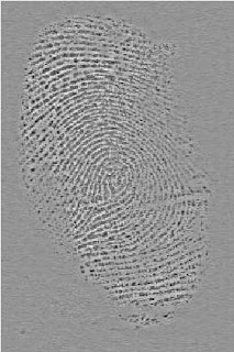
We multiplied this filter with the original FFT of the fingerprint image. After this, we again get its FFT to get the following enhanced image.

The FFT of the enhanced image is shown below. The lower frequencies were removed thereby resulting to enhancement of the higher frequencies.

We then tried using a high-pass binary filter shown below.

The resulting image is shown below.

b) Lunar Landing Scanned Picture: Line Removal

The two groups of irregularly shaped craters north and west of the landing site are secondaries from Sabine Crater. This view was obtained by the unmanned Lunar Orbiter V spacecraft in 1967 prior to the Apollo missions to the Moon. The black and white film was automatically developed onboard the spacecraft and subsequently digitized for transmission to Earth. The regularly spaced vertical lines are the result of combining individually digitized 'framelets' to make a composite photograph and the irregularly-shaped bright and dark spots are due to nonuniform film development. [NASA Lunar Orbiter photograph]

By filtering in the Fourier domain, we can remove the vertical lines present in this image. We first get its FFT.

Using the hints from http://www.roborealm.com/help/FFT.php, we designed a filter mask such that the peaks which lie horizontally along the center of the FFT image will be suppressed. These peaks corresponds to the strong vertical lines in the original image. The filter mask we designed is shown below.

This mask is then multiplied to the FFT of the original image to get the following enhanced FFT.

From this enhanced FFT, we obtain the following enhanced image which obviously has no vertical lines present. Clearly, the image was enhanced.

-o0o-
Collaborators:
Jeric Tugaff for the FFT discussions and hints on filtering in the Fourier space.
Cole Fabros, Benj Palmares and Ed David for the FFT discussions.

-o0o-
Rating:
I give myself an 8/10 because
1. I'm not satisfied with my fingerprint enhancement algorithm. SciLab's mkfftfilter seems not suitable for this job.
2. I'm happy with the results of the Lunar Image tho, we had a hard time figuring how to do it properly. I'm thankful for Jeric's resourcefulness for he found hints in the internet.